Network Analysis of Emotions
In this month’s post, I set out to create a visual network of emotions. Emotion Dynamics tells us that different emotions are highly interconnected, such that one emotion morphs into another and so on. I’ll be using a large dataset from an original study published in PLOS ONE by Trampe, Quoidbach, and Taquet (2015). Thanks to Google Dataset Search, I was able to locate this data. The data is collected from 11,000 participants who completed daily questionnaires on the emotions they felt at a given moment. The original paper is fascinating and I highly encourage checking it out - not to mention that the author’s analysis is the inspiration for this post. The raw data can be freely accessed from the author’s OSF page (link in online article) - props to them for publishing the data!
What is a network? In a sentence, a network is a complex set of interrelations between variables. Some terminology: nodes are the variables (in this case, emotions), and edges are the relationships between the variables. Networks can be directed, which means that variables are linked in a sequence (e.g, from emotion A to emotion B), or undirected, which just shows the relationships. Trampe et al. (2015) created an undirected network in their paper, but the data also allows for a directed network - and this is what I’m going to make for this post.
First, I’ll read in the data and fix up a few spelling errors from the original dataset.
library(tidyverse)

emotion_raw <- read_csv("https://osf.io/e7uab/download") %>%
  rename(Offense = Ofense,
         Embarrassment = Embarassment)

emotion_raw
## # A tibble: 69,544 x 21
## id Hours Day Pride Love Hope Gratitude Joy Satisfaction Awe
## <dbl> <dbl> <dbl> <dbl> <dbl> <dbl> <dbl> <dbl> <dbl> <dbl>
## 1 1 1 3 0 0 0 0 0 0 0
## 2 1 14 1 0 0 0 0 0 0 0
## 3 1 14 2 0 0 0 0 0 0 0
## 4 1 14 4 0 0 0 0 0 0 0
## 5 1 15 3 0 0 0 0 0 0 0
## 6 1 15 3 0 0 0 0 0 0 0
## 7 1 19 1 0 0 0 0 0 0 0
## 8 8 8 5 0 0 0 0 1 0 0
## 9 8 9 2 0 0 0 0 1 0 0
## 10 8 10 7 0 0 0 0 0 0 0
## # … with 69,534 more rows, and 11 more variables: Amusement <dbl>,
## # Alertness <dbl>, Anxiety <dbl>, Disdain <dbl>, Offense <dbl>, Guilt <dbl>,
## # Disgust <dbl>, Fear <dbl>, Embarrassment <dbl>, Sadness <dbl>, Anger <dbl>The data is formatted as a sparse matrix (lots of zeros). We have participant id, Day, and Hour that the emotion was reported. To make this data network compatible, I need to wrangle it into a dataframe of edges - that is a from column and a to column. This will become more apparent shortly.
I can use the function gather to turn the data into long format. By filtering for values of 1, I remove all the zeros from the sparse matrix and I’m left with a column that includes the emotion that was experienced at the time of reporting.
emotion_long <- emotion_raw %>%
  gather(emotion_type, value, Pride:Anger) %>%
  arrange(id, Day) %>%
  filter(value == 1) %>%
  select(-value)

emotion_long
## # A tibble: 187,426 x 4
## id Hours Day emotion_type
## <dbl> <dbl> <dbl> <chr>
## 1 1 19 1 Offense
## 2 1 19 1 Sadness
## 3 1 14 2 Disgust
## 4 1 15 3 Alertness
## 5 1 15 3 Anxiety
## 6 1 15 3 Embarrassment
## 7 1 15 3 Sadness
## 8 1 14 4 Alertness
## 9 1 14 4 Embarrassment
## 10 8 9 2 Joy
## # … with 187,416 more rowsStill, there are no edges here - no link between one emotion and the next. Because the data is arranged so that each subsequent row is the next emotion, I can create a new variable, second_emotion, that is the lead of the emotion in that row. Then, I make sure to remove the last row from each participant id (otherwise there would be a relationship between Participant #1’s last emotion and Participant #2’s first emotion).
emotion_edges <- emotion_long %>%
  mutate(second_emotion = lead(emotion_type)) %>%
  rename(first_emotion = emotion_type) %>%
  select(id, Day, Hours, first_emotion, second_emotion) %>%
  group_by(id) %>%
  slice(-length(id))

emotion_edges
## # A tibble: 175,480 x 5
## # Groups: id [11,332]
## id Day Hours first_emotion second_emotion
## <dbl> <dbl> <dbl> <chr> <chr>
## 1 1 1 19 Offense Sadness
## 2 1 1 19 Sadness Disgust
## 3 1 2 14 Disgust Alertness
## 4 1 3 15 Alertness Anxiety
## 5 1 3 15 Anxiety Embarrassment
## 6 1 3 15 Embarrassment Sadness
## 7 1 3 15 Sadness Alertness
## 8 1 4 14 Alertness Embarrassment
## 9 8 2 9 Joy Alertness
## 10 8 2 9 Alertness Alertness
## # … with 175,470 more rowsNotice how first and second emotion form a sort of chain - Offense to Sadness, Sadness to Disgust, Disgust to Alertness, etc.
We’re ignoring the fact that people are experiencing multiple emotions at once and in those instances we don’t know which emotion was experienced first.
Now that we have our edges, we need to create an object containing the nodes. This is pretty simple, but I’ll add some information indicating the valence and frequency (n) of each emotion, which will help with the visualizations that follow.
emotion_nodes <- emotion_long %>%
  count(emotion_type) %>%
  rowid_to_column("id") %>%
  rename(label = emotion_type) %>%
  mutate(valence = ifelse(label %in% c("Awe", "Amusement", "Joy", "Alertness",
                                              "Hope", "Love", "Gratitude", "Pride",
                                              "Satisfaction"), "positive", "negative"))

emotion_nodes
## # A tibble: 18 x 4
## id label n valence
## <int> <chr> <int> <chr>
## 1 1 Alertness 17932 positive
## 2 2 Amusement 11136 positive
## 3 3 Anger 6394 negative
## 4 4 Anxiety 19115 negative
## 5 5 Awe 3830 positive
## 6 6 Disdain 682 negative
## 7 7 Disgust 7412 negative
## 8 8 Embarrassment 3000 negative
## 9 9 Fear 3457 negative
## 10 10 Gratitude 7379 positive
## 11 11 Guilt 3500 negative
## 12 12 Hope 16665 positive
## 13 13 Joy 23465 positive
## 14 14 Love 18625 positive
## 15 15 Offense 3160 negative
## 16 16 Pride 9214 positive
## 17 17 Sadness 13460 negative
## 18 18 Satisfaction 19000 positiveWe now have an object containing our nodes and an object containing our edges. Now it’s a matter of weighting (counting) the relationships between the emotions.
emotion_network <- emotion_edges %>%
  group_by(first_emotion, second_emotion) %>%
  summarize(weight = n()) %>%
  ungroup() %>%
  select(first_emotion, second_emotion, weight)
## `summarise()` has grouped output by 'first_emotion'. You can override using the `.groups` argument.emotion_network## # A tibble: 315 x 3
## first_emotion second_emotion weight
## <chr> <chr> <int>
## 1 Alertness Alertness 6191
## 2 Alertness Amusement 97
## 3 Alertness Anger 214
## 4 Alertness Anxiety 4784
## 5 Alertness Awe 14
## 6 Alertness Disdain 82
## 7 Alertness Disgust 544
## 8 Alertness Embarrassment 208
## 9 Alertness Fear 109
## 10 Alertness Gratitude 70
## # … with 305 more rowsA few more modifications are needed to make it ready for visualization. I’m trimming some of the really high values using ifelse, just so that they don’t overwhelm the plotting screen.
edges <- emotion_network %>%
  left_join(emotion_nodes, by = c("first_emotion" = "label")) %>%
  rename(from = id)

edges <- edges %>%
  left_join(emotion_nodes, by = c("second_emotion" = "label")) %>%
  rename(to = id) %>%
  select(from, to, weight) %>%
  mutate(weight = ifelse(weight > 4500, 4500, weight))

edges
## # A tibble: 315 x 3
## from to weight
## <int> <int> <dbl>
## 1 1 1 4500
## 2 1 2 97
## 3 1 3 214
## 4 1 4 4500
## 5 1 5 14
## 6 1 6 82
## 7 1 7 544
## 8 1 8 208
## 9 1 9 109
## 10 1 10 70
## # … with 305 more rowsWe need the tidygraph and ggraph packages for the visualization. I’ll note that there are a number of packages for visualizing networks, but ggraph seems to be preferred because it is compatible with ggplot terminology. The function tbl_graph will take the nodes and edges and make them ggraph ready.
library(tidygraph)
library(ggraph)

network <- tbl_graph(emotion_nodes, edges, directed = TRUE)

set.seed(190318)

ggraph(network, layout = "graphopt") +
  geom_edge_link(aes(width = weight, color = scale(weight), alpha = weight), check_overlap = TRUE) +
  scale_edge_color_gradient2(low = "darkgrey", mid = "#00BFFF", midpoint = 1.5, high = "dodgerblue2") +
  scale_edge_width(range = c(.2, 1.75)) +
  geom_node_label(aes(label = label, fill = valence), size = 4) +
  scale_fill_manual(values = c("#FF6A6A", "#43CD80")) +
  theme_graph() +
  theme(legend.position = "none", plot.background = element_rect(fill = "black"))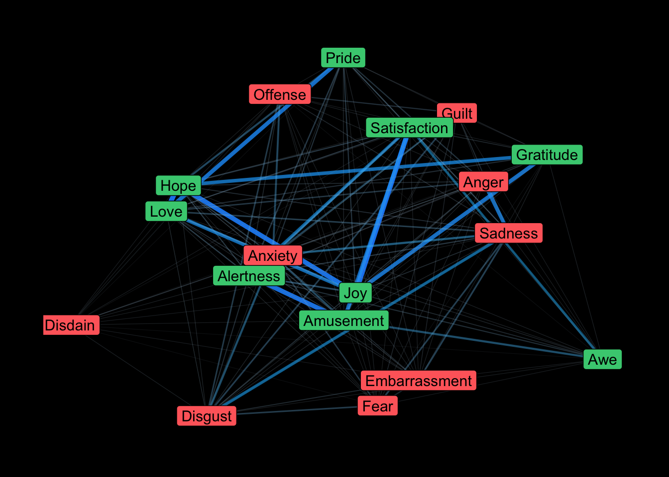
Stronger relationships show up as thicker lines. Positive emotions seem to be more pronounced and interconnected, which is what was found in the original article. Unfortunately, we don’t get a good sense of temporality (adding directional arrows creates more of a mess than anything). An interactive plot might be more informative, so let’s try that using networkD3.
library(networkD3)

nodes_d3 <- emotion_nodes %>%
  mutate(id = id - 1,
         n = (scale(n) + 3)^3)

edges_d3 <- edges %>%
  mutate(from = from - 1, to = to - 1,
         weight = ifelse(weight < 600, 0, log(weight)))
It’s VERY important to transform the values to base 0, which is why I’m using mutate -1. networkD3 won’t work on base 1 values.
Again, I’ve made a few adjustments for visualization purposes. Namely, I’m removing relationships that occur less than 600 times and scaling the values somewhat arbitrarily. Of course, this is exploratory analysis, but caution should be taken when interpreting these results. The function forceNetwork takes the nodes and edges specified above and turns them into something beautiful.
forceNetwork(Links = edges_d3, Nodes = nodes_d3, Source = "from", Nodesize = "n",
             Target = "to", NodeID = "label", Group = "valence", Value = "weight", fontFamily = "sans-serif",
             colourScale = JS('d3.scaleOrdinal().domain(["negative", "positive"]).range(["#FF6A6A", "#43CD80"])'),
             opacity = 1, fontSize = 24, linkDistance = 300, linkColour = c("#8DB6CD"),
             arrows = TRUE, zoom = TRUE, bounded = TRUE, legend = TRUE)
## Links is a tbl_df. Converting to a plain data frame.## Nodes is a tbl_df. Converting to a plain data frame.Hovering over the nodes shows the emotion label and its relationships with other emotions. The arrows indicate directionality in time. It’s a good enough graph, although I would like for the labels to show up at all times. I still have lots to learn about network analysis.
As a final note, I’ll mention that I neglected to adjust for the nested structure of the data - emotions nested within hours, days, and participants. This is crucial when conducting formal statistical tests, but should also be accounted for in visualizations.
###References & Resources
This blog post by Jesse Sadler really helped in the initial stages of my learning on network analysis.
Trampe, D., Quoidbach, J., Taquet, M. (2015). Emotions in everyday life. PLOS ONE. https://doi.org/10.1371/journal.pone.0145450